7.3.1. Beam-column Parametric Study
7.3.1.1. Example Summary
In the following example, a parametric study is run on a series of CSA S16 steel beam-columns loaded in strong axis bending and compression. The goal of this study is to determine in what conditions each of the three compression moment interaction equations govern the strength of each beam-columns.
In CSA, three conditions need to be checked when there is compression / moment interaction: cross sectional strength, overall member strength, and lateral torsional buckling strength. In cross sectional strength, the member is checked to ensure it’s cross section does not fail at every point along the beam. In overall member strength, the member is checked to ensures that the total member does not fail compression. Lateral torsional buckling are neglected, but the buckling length is set to one. In lateral torsional buckling strength, the member is checked to ensure it doesn’t buckle. A more detailed explanation of each check is given in the code commentaries, and example Steel Beam-column Design, W.
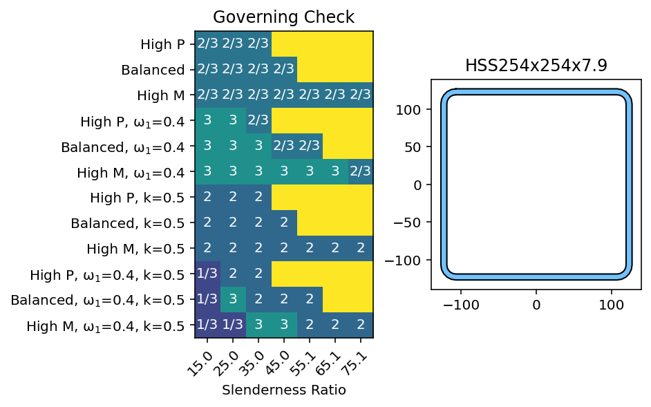
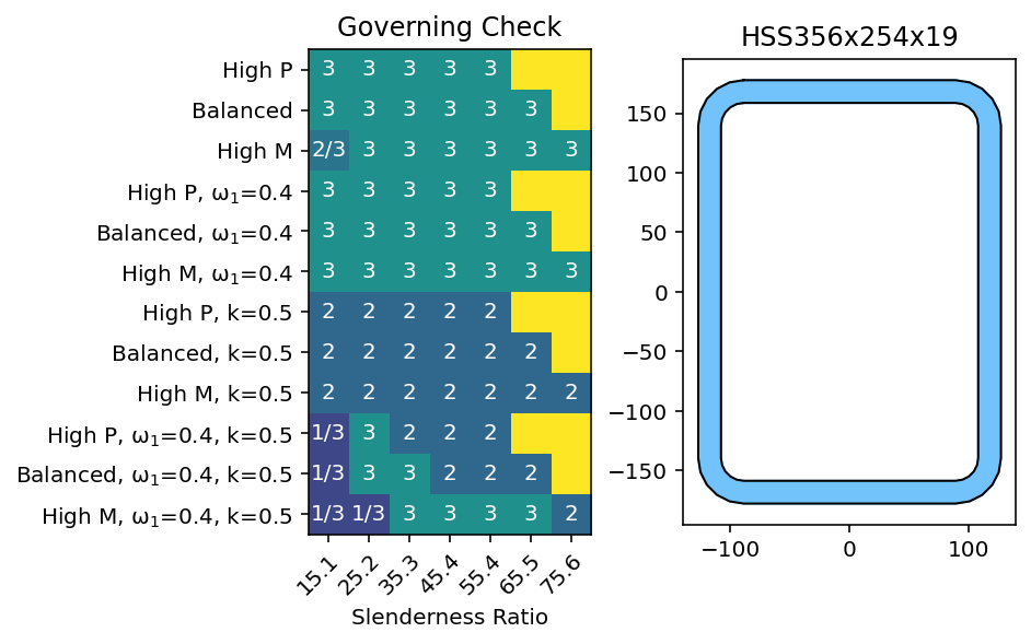
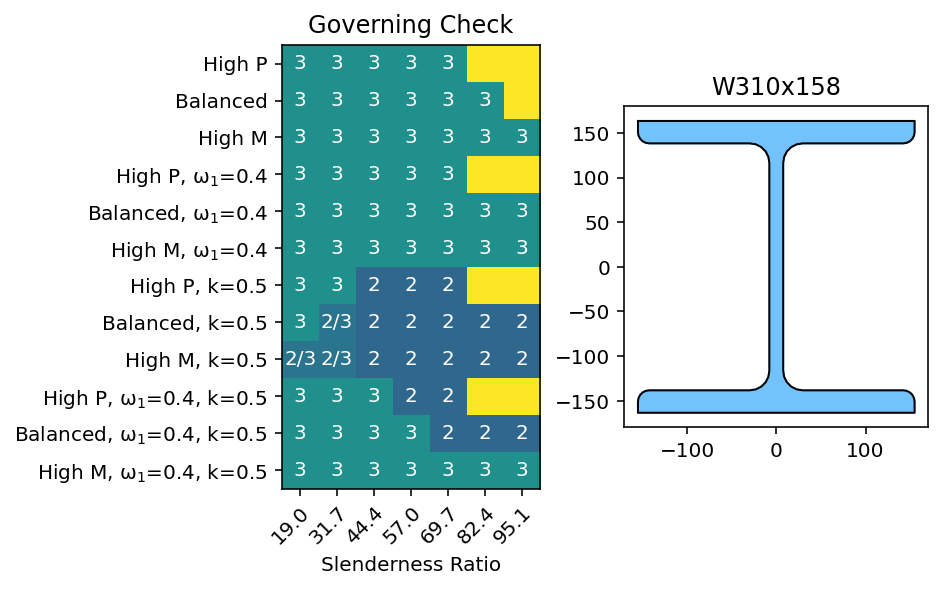
A sample plot of the output is shown below.
7.3.1.2. Problem Setup
Several sections are studied, using different HSS and W profiles. For each section chosen, a total of five input parameters were examined: compression force applied, strong axis moment applied, effective length, load distribution factor, and slenderness. The first two parameters were calculated by deterring the section’s yield compressive strength (Cy) and braced moment resistance (My), then applying a factor to it. For each of the other parameters, three groups are run, with the following factors applied:
High P, where Cf= 0.8Cy, Mf= 0.2My
Balanced, where Cf= 0.5Cy, Mf= 0.5My
High M, where Cf= 0.2Cy, Mf= 0.8My
A total of four cases are considered for the other parameters:
The base case for the analysis is to take k = 1, and the load distribution factor, ω1, is equal to as one. This represents a scenario where moments are always increased for PM interaction, and no interior member bracing is used.
In the second group, ω1=0.4. This represents the best case scenario, where there is a high moment gradient. For low values of slenderness, case 2/3 can have their moments reduced.
In the third group, there is assumed to be buckling restraint at k=0.5. This affects case 3 the most, as the lengths for lateral torsional buckling will be reduced.
In the fourth group, both k=0.5 and ω1=0.4.
Finally, in each analysis group, the effect of slenderness is examined by increasing the sections length from 3m to 15m in increments of 2m. All the above inputs are checked assuming the column is in a braced frame.
7.3.1.3. Code Overview
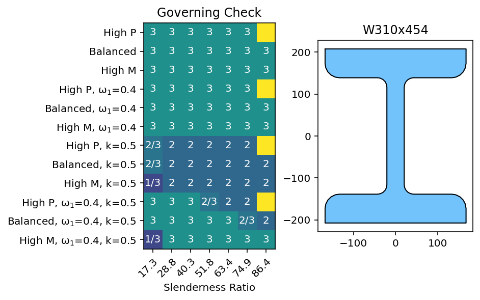
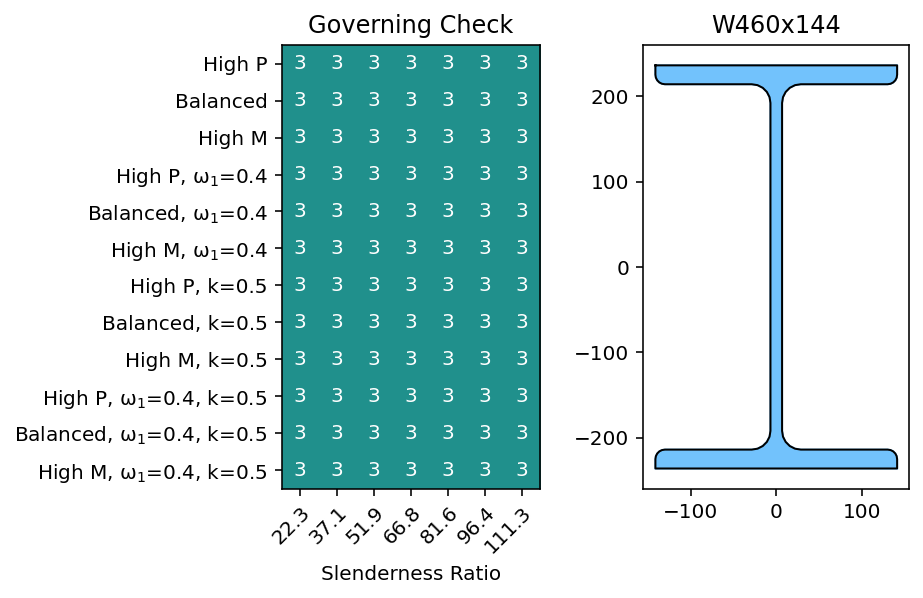
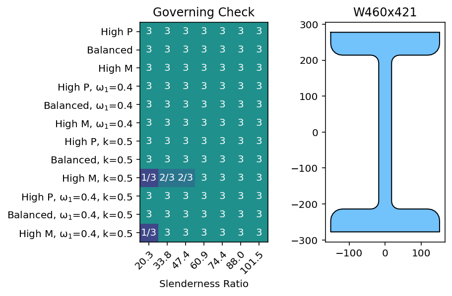
First the necessary libraries and functions are imported. There are two helper functions used in a separate file; one that runs the analysis, and one that makes the plots. Both functions use basic implementations of limitstates and matplotlib. A set of inputs are then defined, and the chosen sections are iterated through. Where two cases have the same utilization, both cases are shown, i.e. 1/3 in a cell means case 1 and 3 are tied. Where the applied load has exceeded the buckling capacity of the column, cells are coloured yellow.
import limitstates as ls
import limitstates.design.csa.s16.c24 as s16

from parametricHelpers import getParametricPlot, runParametericAnalysis

# Set up the material.
mat = s16.MaterialSteelCsa24(345)

# Get a set of members by name.
steelWSections   = ls.getSteelSections(mat, 'csa', 'cisc_12', 'w')
sectionsW310 = ls.filterByName(steelWSections, 'W310')
sectionsW460 = ls.filterByName(steelWSections, 'W460')

steelHssSections  = ls.getSteelSections(mat, 'csa', 'cisc_12', 'hss')
sectionsHss = ls.filterByName(steelHssSections, '254')


# =============================================================================
# Inputs
# =============================================================================

# Define a set of inputs x*Cy, y*Mf, kx, ω1
inputDict = {'High P':                       [0.8, 0.2, 1.0, 1],
             'Balanced':                     [0.5, 0.5, 1.0, 1],
             'High M':                       [0.2, 0.8, 1.0, 1],
             'High P, ${ω_1}$=0.4':          [0.8, 0.2, 1.0, 0.4],
             'Balanced, ${ω_1}$=0.4':        [0.5, 0.5, 1.0, 0.4],
             'High M, ${ω_1}$=0.4':          [0.2, 0.8, 1.0, 0.4],
             'High P, k=0.5':                [0.8, 0.2, 0.5, 1],
             'Balanced, k=0.5':              [0.5, 0.5, 0.5, 1],
             'High M, k=0.5':                [0.2, 0.8, 0.5, 1],
             'High P, ${ω_1}$=0.4, k=0.5':   [0.8, 0.2, 0.5, 0.4],
             'Balanced, ${ω_1}$=0.4, k=0.5': [0.5, 0.5, 0.5, 0.4],
             'High M, ${ω_1}$=0.4, k=0.5':   [0.2, 0.8, 0.5, 0.4]}

# The lengths to use in the analysis.
lengths = [3, 5, 7, 9, 11, 13, 15]

# set up the sections to run the analysis on.
sections = [sectionsW310[1], sectionsW310[11],
            sectionsW460[1], sectionsW460[12],
            sectionsHss[0], sectionsHss[-12], sectionsHss[-3]]
labels = list(inputDict.keys())

# =============================================================================
# Analysis
# =============================================================================

for sec in sections:

    # Run the analysis
    govCases, govUts, slender = runParametericAnalysis(sec, lengths, inputDict)

    # Create the plot using the outputs
    fig, ax = getParametricPlot(sec, slender, labels, govCases, govUts)
def getParametricPlot(section, slendernesses, labels, governingCases, governingUts):
    """
    A helper function to create the parameteric plot.
    """

    Nanalysis = len(labels)
    Nxvalues = len(slendernesses)

    # set up the base plot with two subplots
    fig, ax = plt.subplots(ncols = 2)

    # Define a norm and create an image
    Ncase = 6
    norm = Normalize(vmin=0, vmax=Ncase, clip=False)
    _ = ax[0].imshow(governingCases, norm = norm)

    # Show all ticks and label them with the respective list entries
    ax[0].set_xticks(np.arange(len(slendernesses)), labels=slendernesses)
    ax[0].set_yticks(np.arange(len(labels)), labels=labels)

    # Rotate the tick labels and set their alignment.
    plt.setp(ax[0].get_xticklabels(), rotation=45, ha="right",
             rotation_mode="anchor")

    # Loop over each analysis and create text annotations in each cell.
    for ii in range(Nanalysis):
        for jj in range(Nxvalues):

            # If the force applied is greater than the ,
            # utilization will be very large
            if governingUts[ii, jj] < 10:
                text = _getOutputText(governingCases[ii, jj])
                ax[0].text(jj, ii, text, ha="center", va="center", color="w")

    # Plot the section
    _, ax2 = ls.plotSection(section, ax = ax[1])


    # Set the title for the section
    name = section.name.split(' ')[0]
    ax[1].set_title(name)

    # set up teh title the check plot, and some labels.
    ax[0].set_title("Governing Check")
    ax[0].set_xlabel("Slenderness Ratio")

    plt.show()
    return fig, ax
def runParametericAnalysis(section, lengths, inputDict):
    """
    Run the analysis on each section in the input dictionary.
    """

    # initialize the variables
    governingCases = []
    governingUts   = []

    # Iterate through each analysis input
    for key in inputDict:

        # Extract the input values
        cratio, Mratio, kx, omegax1 = inputDict[key]

        # Initialize containing variables for each input
        trialGoverningCases = []
        trialGoverningUts   = []
        slendernesses       = []

        # A number of different slenderness conditions are checked by using
        # differnt lengths
        for L in lengths:

            # create the beam column using the input variables.
            # It's assumed the brace point will brace both axes.
            beamColumn = s16.getBeamColumnSteelCsa24(L, section,
                                                     kx = kx, ky = kx)

            # Calcualte teh slenderness ratio for the beam
            slenderness = s16.checkElementSlenderness(beamColumn, False)

            # Calcualte the initial applied loads.
            Cr  = s16.checkColumnCr(beamColumn,  lam = 0)
            Cf  = Cr*cratio
            Mp  = s16.checkBeamMrSupported(beamColumn, Cf=Cf)
            Mfx = Mp*Mratio

            # Get the output utilizations.
            u = s16.checkBeamColumnCombined(beamColumn, Cf, Mfx,
                                            omegax1 = omegax1,
                                            isBracedFrame = True)

            # skip the case 3 check
            u = u[:3]

            # Get the governign load combineation
            ind = np.argmax(u)
            ut = np.max(u)

            # find if there are any ties. If there are skip them
            inds = np.where(np.abs(u - ut) < 0.01)[0]
            if len(inds) >=2:
                # print(inds)
                ind = min(inds) + max(inds)/10 +0.1

            # set the outputs
            trialGoverningCases.append(ind)
            trialGoverningUts.append(round(ut,2))
            slendernesses.append(slenderness)

        # Set the output lists for each trial group.
        governingCases.append(trialGoverningCases)
        governingUts.append(trialGoverningUts)

    # Get the final outputs, and
    governingCases = np.array(governingCases) + 1
    governingUts  = np.round(governingUts, 1)

    # remove cases where
    slendernessFailsInds = np.where(10<governingUts)

    governingCases[slendernessFailsInds] = 6

    slendernesses = list(slendernesses)
7.3.1.4. Results
Each plot is shown below. There are a few results immediately noticeable, the biggest being that case 1 did not govern any of the sections alone. This makes sense, case 2 and case 3 will have lower compression or bending resistance than case 1 due to slenderness considerations. Because Case 3 takes 1 <= U1x except when there is negative bending, Case 1 can only govern if there is a high moment gradient, and negative bending.
For W sections, Case 3 almost always governed - the notable exception being where k=0.5 occasionally case 2 governs in squat sections. This also matches expectations, as W sections will have a low torsional stiffness. Sections that are tall generally more prone to buckling around their weak axis, while in squat the difference between Ix and Iy is smaller. Squat sections also have a larger torsional stiffness porportional to their axial / bending resistance.
For HSS sections, rectangular sections are governed by case 3, except where k=0.5. This is likely because in uniaxial bending, case 2 only checks buckling of the column in it’s strong axis. For square sections case 2/3 have similar capacities. This also matches expectation, as the strong and weak axis compression strength will be the same. HSS members were more likely to fail in pure compression.
In all sections, those that started with high compression resistance were more likely to exceed the buckling force at high slenderness values.
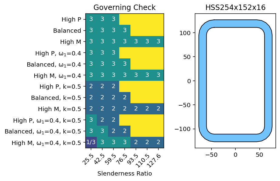
7.3.1.5. Closing Thoughts
Based on the observed outcomes and explaination given above, if there is only positive bending and no intermediate bracing, case 3 will govern W sections and HSS Sections. Members with intermediate bracing are more likely to be governed by case 2, but only if they have a relatively high torsion resistance, or similar comrpession resistance in both it’s strong / weak direction.